All About Diffusion
Introduction
Like many others, I’ve long been familiar with the technology of diffusion, especially within the last few years with the introduction and subsequent advancements of AI-generated art and video. It is, however, only recently when I’ve really dived deep into the theory behind the technology. And while it has been a lot of math to chew, I eventually got through the thicker parts of the story and I now believe that I have enough of a sufficient understanding of the bigger picture to explain it. So this article serves as a documentation of the notes that I’ve taken as I’ve stepped through the parts of the CS 180 project 5 as well as an internalization of the lessons I’ve learned along the way.
Some excellent resources that helped me understand diffusion:
- But how do AI images and videos actually work? - 3b1b
- Denoising Diffusion Probabilistic Models
- An Introduction To Flow Matching
Problem Background
At a high level, we can frame generative modelling as modelling a distribution of interest $q_1(x)$, which has an unknown density given a sample of vectors from that density $x_1, x_2, \dots, x_n$. We use these samples to learn to approximate the distribution $q_1(x)$ well enough to sample new points from this high-dimensional distribution efficiently. Specifically with the case of modelling images, our distribution $q_1$ can be referred to as the image manifold that all images live on, and the sample of vectors $x_1, x_2, \dots, x_n$ is the dataset that we train our generative diffusion model off of.
Many classes of generative models prior to diffusion models have tackled variations of the generative modelling problem from the restricted boltzman machines (RBM) pioneered by the famous computer scientist Geoffrey Hinton to generative adverserial nets (GAN) of the 2010s. The background of the more recent approach of diffusion modelling is very interesting, however, being inspired the methods of non-equilibrium statistical physics.

The 2015 paper Deep Unsupervised Learning using Nonequilibrium Thermodynamics provided the core idea of using techniques from physics to create a model that could turn data into noise and then reverse the process turning noise back into data. The 2019 paper Generative Modeling by Estimating Gradients of the Data Distribution introduced a different, but related, approach using score-based generative models produced with Langevin dynamics using the gradients of data distributions. Then the landmark paper Denoising Diffusion Probabilistic Models combined both of these approaches, demonstrating that diffusion models could achieve image quality comparable to state of the art GANs at the time.
Diffusion Primer
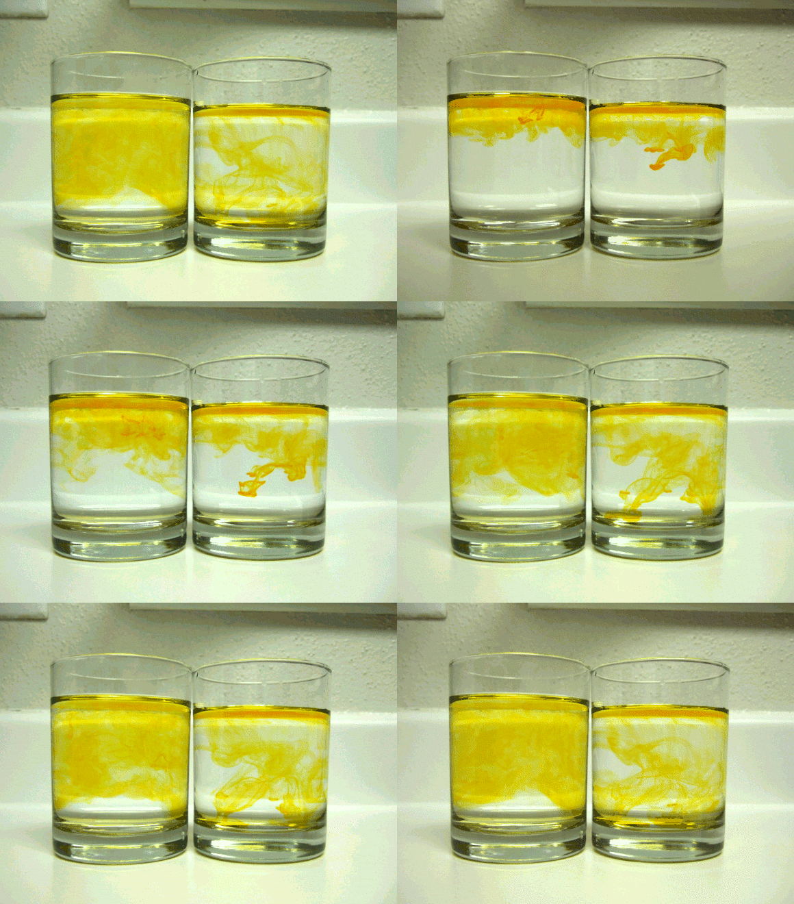 source: What is diffusion?
From physics, diffusion can be defined as the net movement of a substance from a region where it is more highly concentrated to a region where it is less concentrated produced due to random interactions of molecules. According to the kinetic theory of matter, all atoms and molecules are in constant random motion. As these molecules are excited, they interact with adjacent substances, bouncing off of them and spreading them around. The simple diffusion of a specific substance into water shown in the figure above shows how molecules of yellow food dye being more concentrated towards the top of the glass when first introduced have a net movement towards the bottom of the glass and as they interact with the water molecules, the molecules of yellow food dye move randomly around the glass until the food coloring and water are evenly mixed: a state of equilibrium. Diffusion modelling applies a mathematical model to this phenomenon, in the form of a continuous-time Markov Chain, as shown below:

At its core, diffusion models involve a forward process and a backwards process. The forward process involves taking steps into the future probabilistically from a starting state $x_0$ and adding small amounts of noise in the opposite direction of sampling until the result is pure Gaussian noise $x_T$. The backwards process is the complete opposite, starting from a state of complete noise $x_T$ an gradually reversing the noise added in small amounts until we recover a signal $x_0$.
The diffusion model learns to reverse the forward process, learning the parameters of the reverse process. Given a noisy image $x_t$ at some time step $t$, it predicts the noise in the image. The predicted noise can then be used to remove noise from the image to estimate $x_0$ in one step or remove a portion of the noise to obtain an estimate of $x_{t-1}$.
To sample images from the parameterized reverse diffusion process, we start with a completely noisy $x_T$ at timestep $T$, and then take small incremental steps backwards from $T$, predicting the noise to remove to estimate $x_{T-1}$, and so on until we reach an clean, noise-free image that belongs on the image manifold $x_0$. For the original paper DDPM, the authors paramaterized $T=1000$. The noise added at each step is determined by some schedule of parameters $\beta_1, \beta_2, \dots, \beta_T$. Which can also be parameterized by $\alpha_t$ variables with the formula $\alpha_t = 1 - \beta_t$. The authors of the DDPM paper chose this schedule to be evenly interpolated from $\beta_1 = 10^{-4}$ to $\beta_T = 0.02$ over $T=1000$ timesteps for the purposes of ensuring the forward and reverse processes have the same approximate functional form.
This means that, although the forward process could have also been parameterized, they chose to deterministically destroy an image into pure noise and focus modelling the interesting part of the problem: the reverse process. The authors represented the reverse process with a U-Net backbone, inspired by the previous work with PixelCNN++
The Forward Process
The forward process is fixed to a Markov chain that gradually adds Gaussian noise to data with schedule $\beta_1, \dots, \beta_T$:
$$ q(x_t | x_{t-1}) := \mathcal{N}(x_t; \sqrt{1-\beta_t} x_{t-1}, \beta_t \mathbf{I}) $$
$$ q(x_{1:T} | x_0) := \prod_{t=1}^T q(x_t | x_{t-1}) $$
The forward process variances $\beta_t$ are chosen by the authors to be held constant as small hyperparameters, because both processes have the same functional form with this condition. Additionally, the $\beta$ s are increasing at a slow but steady rate creating the effect of more aggresively adding noise as $t$ gets closer to $T$.
The DDPM authors note an interesting property of the forward process: sampling $x_t$ at an arbitrary timestep $t$ has a closed form given $x_0$. With $\alpha_t := 1 - \beta_t$ and $\bar{\alpha_t} := \prod_{s=1}^t \alpha_s$, we can sample $q(x_t | x_0)$
$$ q(x_t | x_0) = \mathcal{N}(x_t; \sqrt{\bar{\alpha}_t} x_0, (1-\bar{\alpha}_t) \mathbf{I}) $$
This can then be represented in a more digestible form with
$$ x_t = \sqrt{\bar{\alpha_t}} x_0 + \sqrt{1-\bar{\alpha_t}} \epsilon \quad \text{for} \quad \epsilon \sim \mathcal{N}(0, \mathbf{I}) $$
DeepFloyd Model
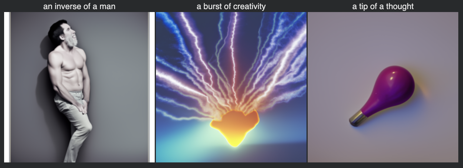
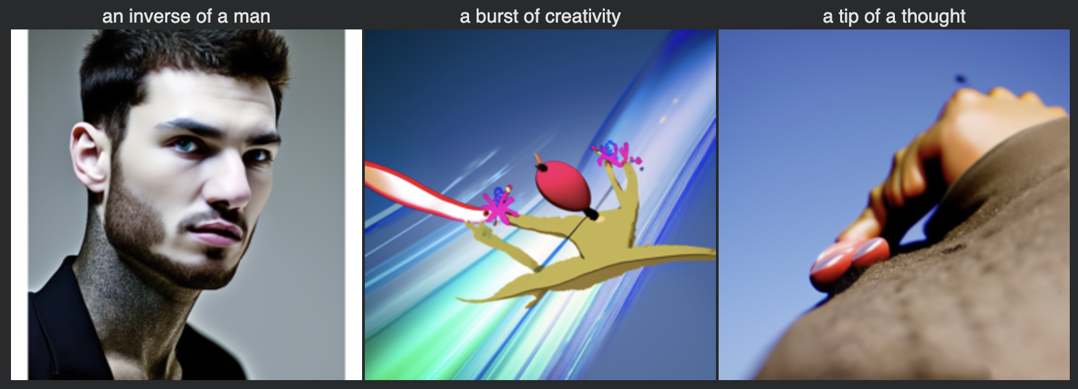
Based on project description, I used the pretrained DeepFloyd text-to-image model, which takes text prompts as inputs and outputs images aligned with text. Converting raw string prompts into an embedding vector as a deterministic numerical representation of text that exists in a high-dimensional latent semantic space, however, is a necessary prerequisite to run inference on the model. Interested in seeing what I could generate out of this model, I came up with 3 interesting prompts amongst others that were provided to test out the limits of DeepFloyd:
- ‘a burst of creativity'
- ‘an inverse of a man'
- ‘a tip of a thought’
Using a torch seed of 100 across all of my implementations, I generated prompt embeddings with an existing text embedding model and ran inference with 10 and 20 inference steps:
Implementing the forward process
I used the schedule of $\bar{\alpha_1}, \dots, \bar{\alpha_T}$ provided by the DeepFloyd authors to implement the forward process,
    def forward(im, t):
      """
      Args:
        im : torch tensor of size (1, 3, 64, 64) representing the clean image
        t : integer timestep

      Returns:
        im_noisy : torch tensor of size (1, 3, 64, 64) representing the noisy image at timestep t
      """
      with torch.no_grad():
        alpha_t = torch.sqrt(alphas_cumprod[t])
        beta_t = torch.sqrt(1 - alphas_cumprod[t])
        eps = torch.randn_like(im)

        im_noisy = alpha_t * im + beta_t * eps

      return im_noisy
Here are the results of noise added to an image of the Campinile tower on the Berkeley campus at different timesteps:

The Reverse Process
Let $p_{\theta}(x_0) := \int p_{\theta}(x_{0:T}) dx_{1:T}$. For latent $x_1, \dots, x_T$ images of the same dimensionality as the data $x_0 \sim q(x_0)$, the joint distribution $p_{\theta}(x_{0:T})$ is known as the reverse process, defined as a Markov chain with learned Gaussian transitions starting at $p(x_T) = \mathcal{N}(x_T; 0, I)$:
$$ p_{\theta}(x_{t-1} | x_t) := \mathcal{N}(x_{t-1}; \mu_{\theta}(x_t, t), \sum_{\theta}(x_t, t)) $$
$$ p_{\theta}(x_{0:T}) := p(x_T) \prod_{t=1}^T p_{\theta}(x_{t-1} | x_t) $$
The authors of DDPM set the $\sum_{\theta}(x_t, t) := \sigma_t^2 I$ where $\sigma_t^2$ is taken to be their choice of untrained time-dependent constant values of variance. Experimentally, they used both $\sigma_t^2 = \beta_t$ and $\sigma_t^2 = \tilde{\beta_t} = \frac{1 - \bar{\alpha_{t-1}}}{1 - \bar{\alpha_t}} \beta_t$, finding both to yield similar results. For future parts of this implementation, neither of the choices of $\sigma_t^2$ are really relevant because we have our U-net model output an estimate of the variance as well as an estimate of the noise present in image $x_t$, $\epsilon_{\theta} (x_t, t)$.
The main part of the formula, the $\mu_{\theta}$ represents an approximation of $\tilde{\mu_t}$, a function that takes in the current image $x_t$ and the time $t$ and outputs an estimate of the average of all potential $x_{t-1}$s. After some analysis of the loss function of $L_t$ based on $p_{\theta}(x_{t-1} | x_t) = \mathcal{N}(x_{t-1}; \mu_{\theta}(x_t, t), \sigma_t^2 I)$, they use parameterizations of $x_t (x_0, \epsilon) = \sqrt{\bar{\alpha_t}} x_0 + \sqrt{1 - \bar{\alpha_t}} \epsilon$ for $\epsilon \sim \mathcal{N}(0, I)$ to derive an estimate of $x_0$ and their sampling formula $\mu_{\theta}$ which relies entirely upon inputs $x_t$ and $t$:
$$ x_0 \approx \frac{x_t - \sqrt{1 - \alpha_t} \epsilon_{\theta}(x_t, t)}{\sqrt{\alpha_t}} $$
$$ \mu_{\theta}(x_t, t) = \frac{1}{\sqrt{\alpha_t}} (x_t - \frac{\beta_t}{\sqrt{1 - \bar{\alpha_t}}} \epsilon_{\theta} (x_t, t)) $$
where $\epsilon_{\theta}$ is what the diffusion model U-net outputs given input of $x_t$. The first formula will be useful for our one-step denoising trials, and the iterative denoising formula and its equivalent more easily implemented form follows:
$$ x_{t-1} = \frac{1}{\sqrt{\alpha_t}} (x_t - \frac{\beta_t}{\sqrt{1 - \bar{\alpha_t}}} \epsilon_{\theta} (x_t, t)) + \sigma_t z \quad \text{for} \quad z \sim \mathcal{N}(0, I) $$
$$ x_{t-1} = \frac{\sqrt{\bar\alpha_{t-1}}\beta_t}{1 - \bar\alpha_t} x_0 + \frac{\sqrt{\alpha_t}(1 - \bar\alpha_{t-1})}{1 - \bar\alpha_t} x_t + v_\sigma $$
For the second formula, it is important that one uses the approximation of $x_0$ shown above and note that the $v_\sigma$ is also predicted in addition to the $\epsilon_\theta$ by the DeepFloyd U-net implementation and results that follow.
Classical Denoising
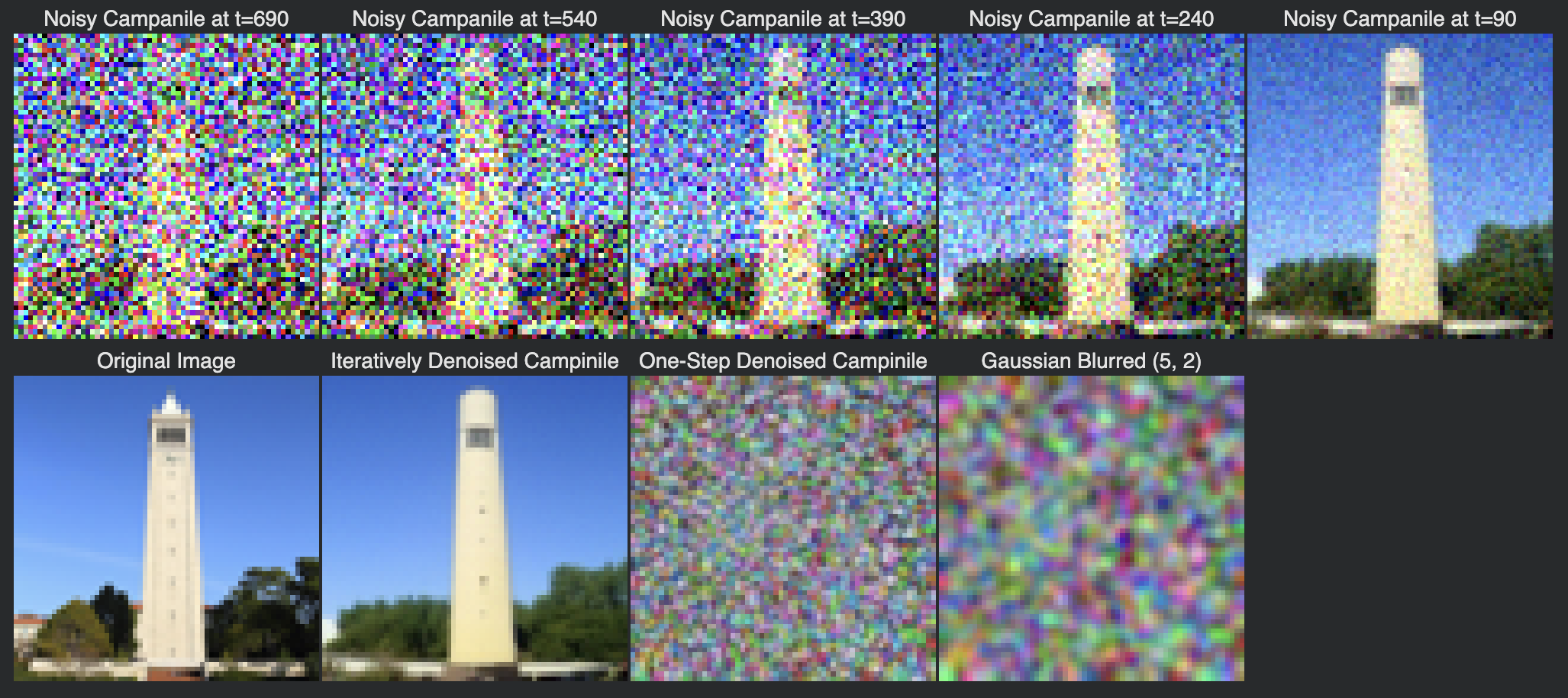
Classical Denoising involves using a low-pass Gaussian filter to filter out the high-frequency noise in the image. The results of classical filtering on our noisy images of the campinile can be seen:

One-Step Denoising
One-step denoising involves using our formula for the estimate of $x_0$ given inputs $x_t$ and $t$. The U-Net was trained with text conditioning, so we’ll use a prompt embedding for the prompt “a high quality photo” to guide the outputs of the U-Net. The following are results shown for different time_steps:
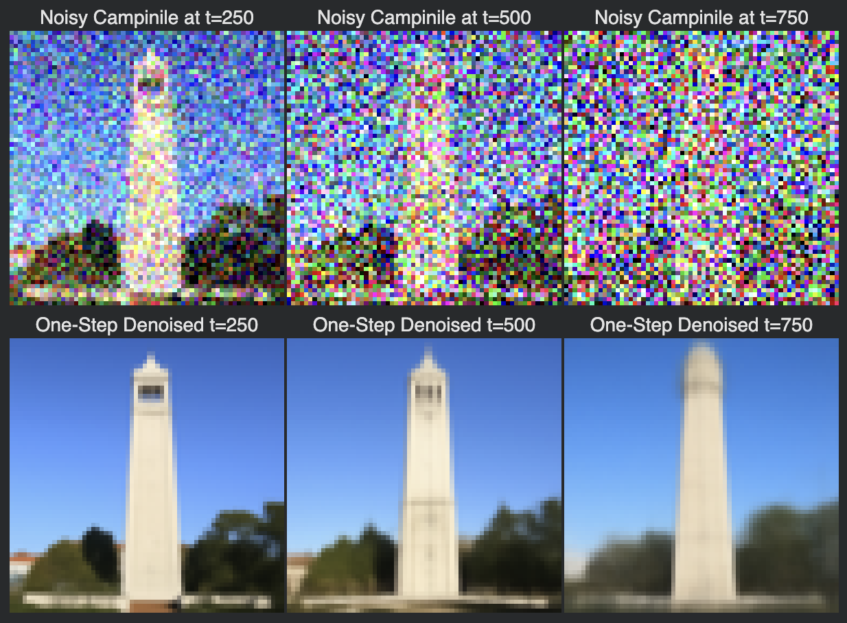
The results are drastically better than the results of classical denoising, however for greater timesteps and a noisier starting $x_t$, the results of one-step denoising are not as good. The results can be improved with iterative denoising.
Iterative Denoising
Using the second formula for iterative denoising and our one-step denoising estimate of $x_0$, the results of iterative denoising are shown at various timesteps along the process, along with the final results compared between the original image, the iteratively denoised result, the one-step denoised campinile, and the gaussian blurred version of it. This time, I use an initial starting time of $t=690:
Diffusion Model Sampling
Using pure noise an the same prompt embedding for “a high quality photo”, we can set up a sampling loop by setting $t=990$ and passing in the starting image $x_990$ as pure Gaussian noise to input into our iterative denoising process. So, we are effectively denoising pure noise to images that exist on the image manifold. The results show what that looks like:

Classifier Free Guidance
The results of the sampling process can be improved with a technique called Classifier-Free Guidance. With CFG, we compute an estimate of noise conditioned on a text prompt, and an estimate of noise without a text prompt. We denote these as $\epsilon_c$ and $\epsilon_u$. Then the new noise at each step of iterative denoising can be computed as:
$$ \epsilon = \epsilon_u + \gamma(\epsilon_c - \epsilon_u) $$
where $\gamma$ controls the strength of the CFG. For $\gamma=0$, we get an unconditional noise estimate, and for $\gamma=1$, we get the conditional noise estimate. For $\gamma > 1$, we can get much higher quality images, and as of the latest investigations, it is still not entirely known why. Using a scale $\gamma = 7$ and an unconditional prompt embedding for "" and conditional prompt embedding for “a high quality photo”, here are some of the results:

Image-to-image Translation
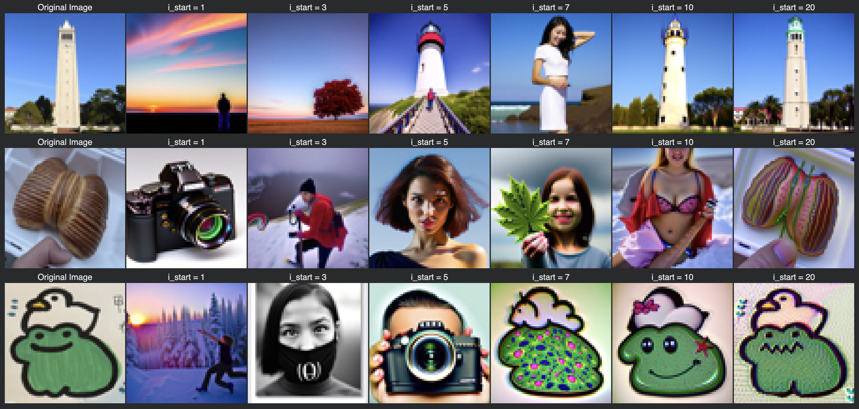
With our iterative denoising process demonstrated on an image of the Campinile, we take a real image, add noise to it, and then denoise. This allows us to make edits to existing images such that the more noise we add, the greater the resulting edits will be. This can be thought of as forcing a noisy image back onto the natural image manifold. Using different noise levels and the conditional text prompt “a high quality photo”, I’ve edited an image of the campinile and two other images:

Here are more results of images taken off of the web and my own hand drawings:


Inpainting
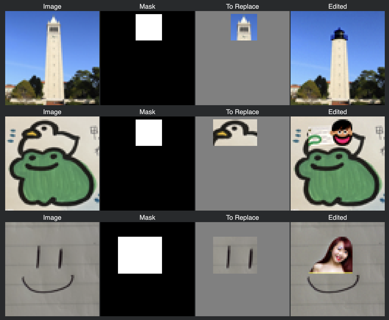
This process can actually be co-opted into procedure for inpainting. So given an image $x_{orig}$ and a binary mask $m$, we create a new image with the same content where $m$ is 0 but new content where $m$ is 1. We run the denoising diffusion loop, but after every step, after obtaining $x_t$ we apply the formula to mask the appropriate areas highlighted for inpainting:
$$ x_t \leftarrow mx_t + (1-m)\text{forward}(x_{orig}, t) $$
Here are some results of this inpainting procedure:
Text-Conditional I2I Translation
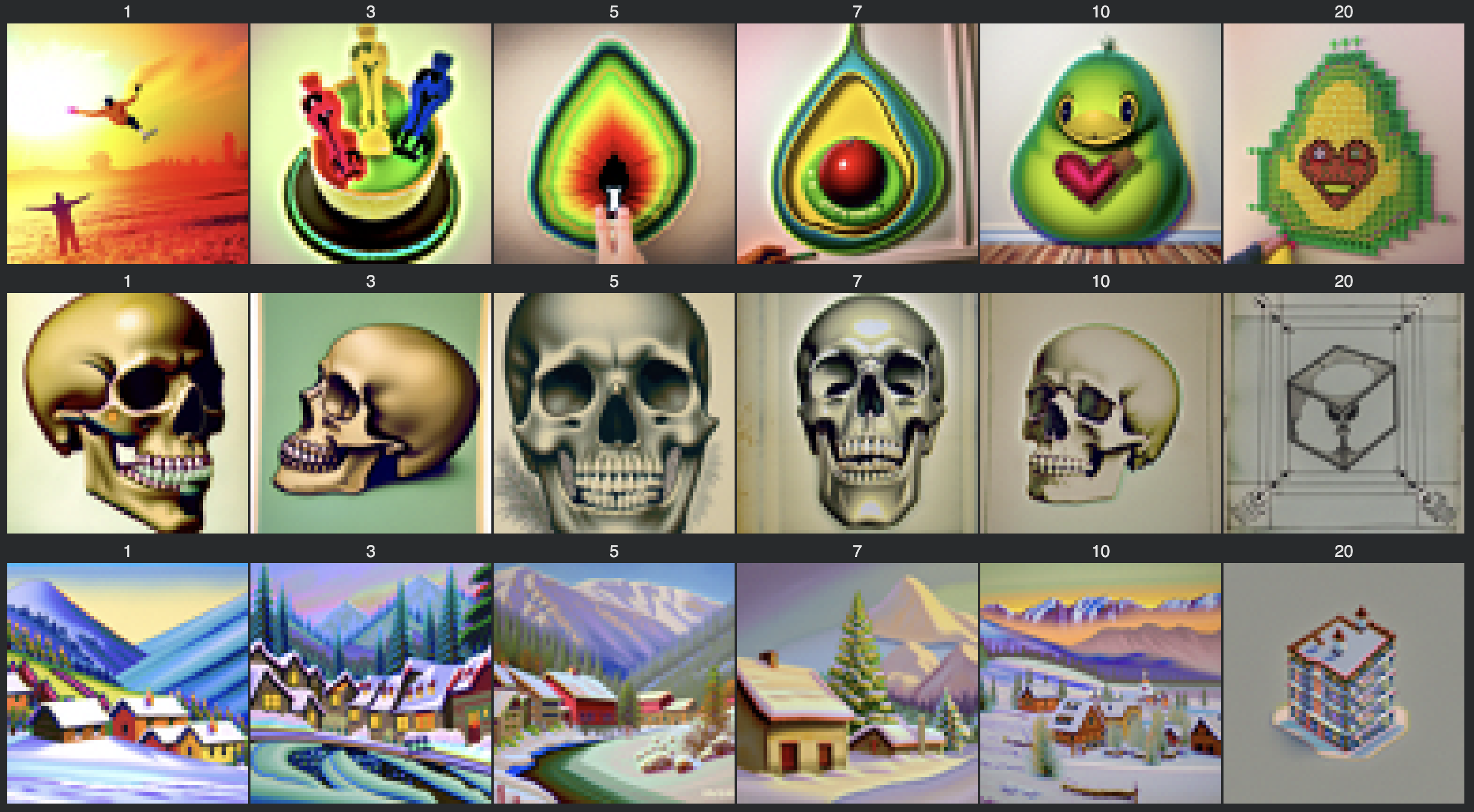
We can also do the same thing for editing existing images but instead of projecting a noisy image back towards the natural image manifold, we add controls on this process with natural language. That is, instead of using the prompt embedding for “a high quality photo” we can change it to anything of our choice. The images shown below are generated out of the prompts of “a burst of creativity”, “a lithograph of a skull”, and “an oil painting of a snowy moountain village”:
Visual Anagrams
Diffusion models can also be used to create optical illusions with a clever manipulation of the estimated noise applied in each iterative denoising step. We first denoise an image $x_t$ at step $t$ normally with prompt $p_1$ to obtain noise estimate $\epsilon_1$. But then, we can flip $x_t$ upide down, and denoise to get noise estimate $\epsilon_2$. Then we flip $\epsilon_2$ and average the two noise estimates.
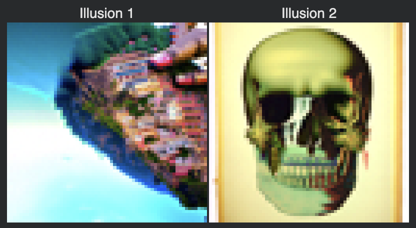
The right image is of a skull but when flipped it is like a waterfall
Hybrid Images
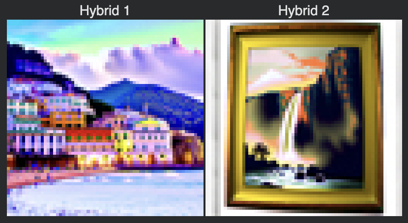
In the nature of visual anagrams and creating optical illusions, we can generate images that when viewed from up close look like one object but when viewed from afar looks like something completely different. We create the composite noise estimate $\epsilon$ by estimating noise with two different prompts $p_1$ and $p_2$, but instead of flipping the noise estimate for the second case, we keep the image right-side up and combine the low frequencies from one noise estimate with the high frequencies of the other noise estimate. Then this noise composite can be used for one cycle of iterative denoising.
2661 Words
2025-11-26 00:00